Understanding Simpson’s Paradox: A Simple Explanation

Simpson's Paradox is a statistical phenomenon where a trend appears in different groups of data but disappears or reverses when these groups are combined. This paradox highlights the importance of considering confounding variables and understanding the causal relationship between variables.
Example Scenario: Work Environment
Let’s consider a hypothetical work environment where the number of women (W) is greater than the number of men (M). However, when looking at the distribution of managerial positions (P), it seems that more men occupy higher-level positions compared to women.
Now, suppose there’s a characteristic Z, representing gender, and you suspect it might influence the choice of assigning a managerial position (P) because a specific time dedicated to a critical task (T) is primarily marketed toward men (M).
To illustrate this paradox, we’ll create synthetic data in R.
Install and load necessary library
Set seed for reproducibility
set.seed(123)Generate synthetic data
Assign managerial positions based on gender and a confounding variable
Create a data frame
Display the initial summary
summary(data) gender count manager
Length:2000 Min. :200 Min. :0.0000
Class :character 1st Qu.:352 1st Qu.:0.0000
Mode :character Median :500 Median :1.0000
Mean :500 Mean :0.5615
3rd Qu.:648 3rd Qu.:1.0000
Max. :800 Max. :1.0000 In this example, we have created a dataset with a larger number of women, but the chance of obtaining a managerial position for men is influenced by a confounding variable. Now, let’s examine the paradox.
Calculate the proportion of managerial positions for each gender
Display the proportions
proportion_table# A tibble: 2 × 2
gender proportion
<chr> <dbl>
1 Men 0.626
2 Women 0.497library(ggplot2)
proportion_table%>%
ggplot(aes(gender,proportion,fill=gender))+
geom_col(color="white",show.legend = F)+
scale_fill_viridis_d()+
labs(title = "Proportion of Managers by Gender",
subtitle = "Example of the Simpson's Paradox",
x="",
caption = "Data: Syntetic | Graphics: Federica Gazzelloni") +
coord_equal()+
ggthemes::theme_pander()+
theme(plot.caption = element_text(hjust = 0.5))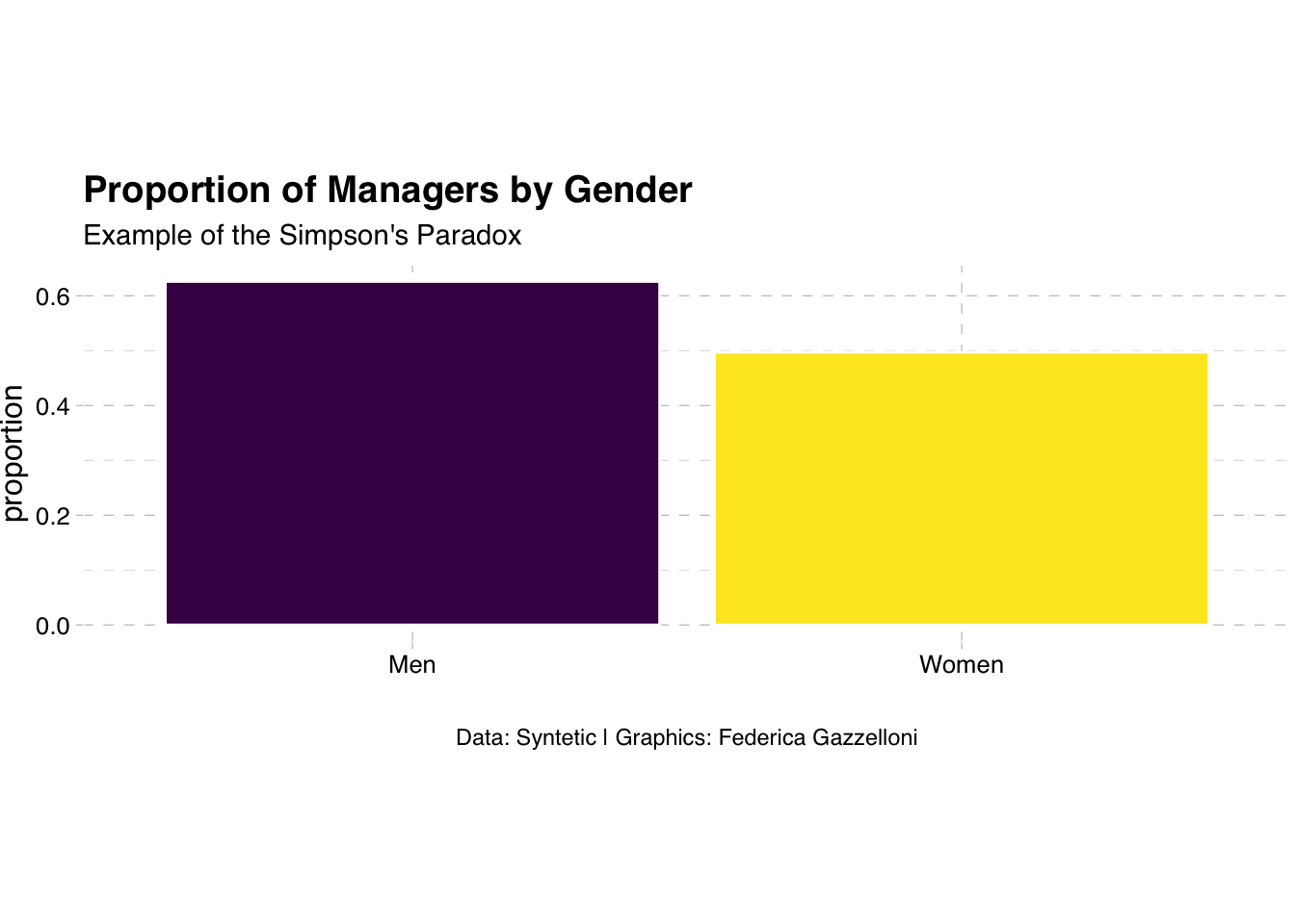
In this scenario, when examining the proportion of managerial positions within each gender group, it might appear that men have a higher chance. However, when we consider the entire dataset, we may find the opposite due to the confounding variable.
The key takeaway is that understanding causation is crucial, and Simpson’s Paradox emphasizes the need to consider confounding factors when interpreting data.